Integrating VPFs into a Holistic Financial Plan

Important Disclosures & Risk Warnings

VPF contracts involve significant risks, including counterparty risk, liquidity risk, and the potential for total loss of the underlying collateral. These strategies are generally intended for sophisticated, high-net-worth investors.

The Monte Carlo simulations presented are hypothetical in nature, do not reflect actual investment results, and are not guarantees of future results. Actual results will vary, perhaps significantly.

This post is for educational purposes only. Always consult with a qualified tax professional before entering into a VPF or Direct Indexing strategy.

I continue to study how advanced tax planning strategies affect financial planning and portfolio risk management. In this blog post we’ll deep dive into risk management when using Variable Prepaid Forward (VPF) contracts.

If you would like to make yourself familiar with VPFs first, I recommend reading our previous posts. They should give you a good overview and prepare for this blog post:

VPF is a complex strategy which affects both portfolio expected returns and volatility. It’s often paired with other strategies such as Long/Short Direct Indexing which intentionally increases idiosyncratic risk within the portfolio to maximize tax-loss harvesting opportunities. This complexity makes answering the question “How much do I need to allocate for my retirement?” more difficult.

Most financial planning software assumes that an investment portfolio is some combination of stocks and bonds with constant standard deviation (volatility). It’s not the case when VPF contracts are used.

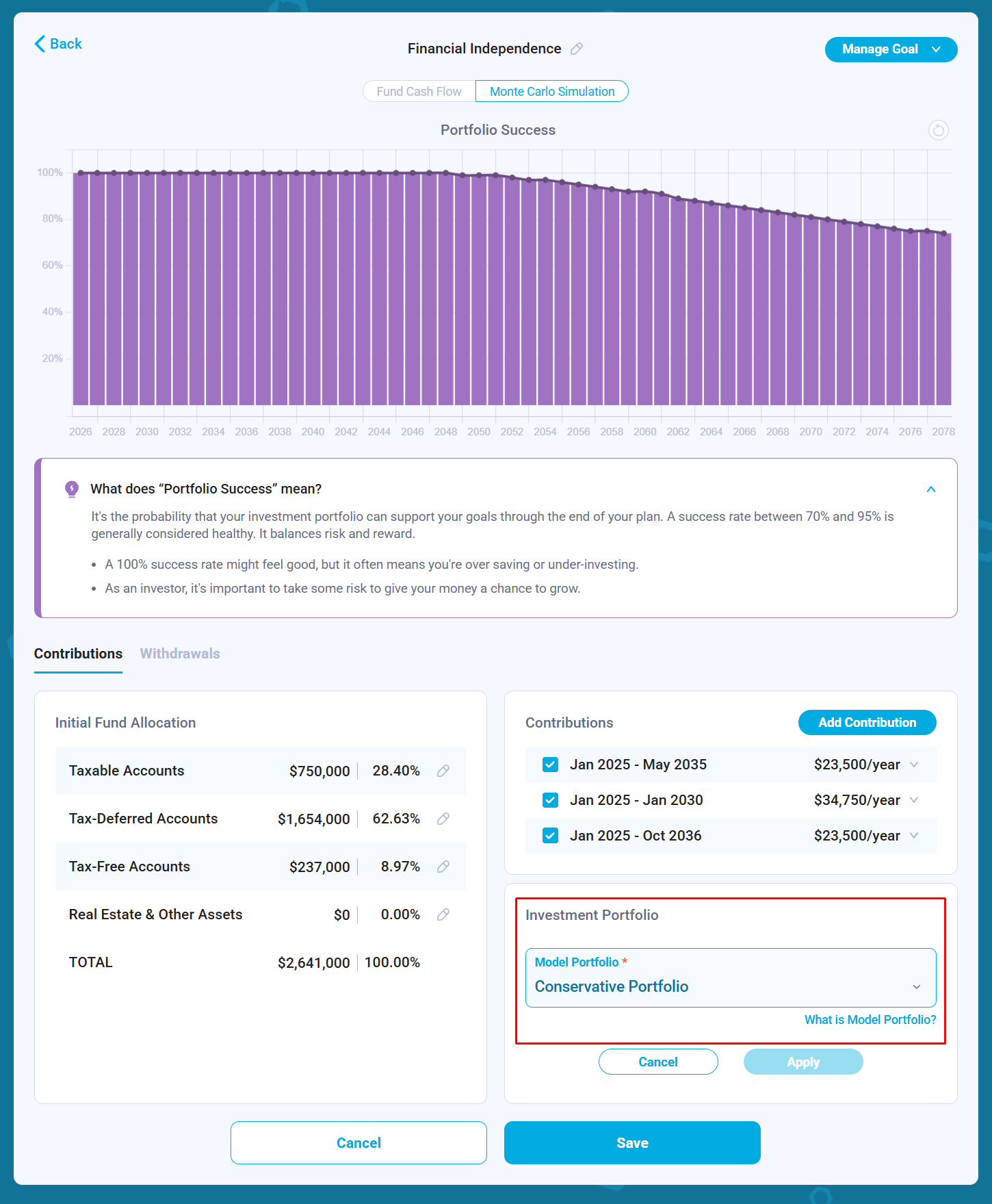
How do we estimate Portfolio Success and decide the initial fund allocation for a retirement fund if we’re enrolled in a VPF contract?

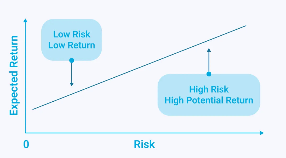
Risk & Returns Tradeoffs

Both portfolio expected returns and volatility affect the size of our retirement portfolio needed to cover our future living expenses:

Higher investment returns allow us to reduce initial fund allocation.
Higher volatility in the portfolio requires us to increase initial fund allocation.

In the accumulation phase, volatility is our friend (dollar-cost averaging, direct indexing), but in retirement, it’s one of the biggest threats. If the market drops while we are working, we simply wait for it to recover. But if the market drops while we are withdrawing funds for our lifestyle, we are effectively “locking in” those losses.

Expected returns and volatility have positive correlation, but the relationship is not linear and complex strategies such as VPF make both expected returns and volatility change over time.

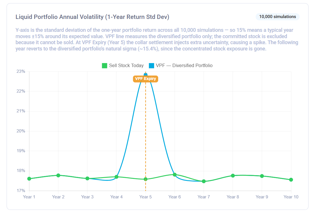
VPF Volatility

In my previous post Analyzing VPFs as a Leveraged Diversification Tool I argued that portfolio volatility is higher during the VPF contract. While it’s true, it’s overall portfolio volatility. It can be ignored because the stock used in the VPF contract is essentially locked and can’t be used to cover living expenses.

It’s only diversified portfolio volatility (money that we invested using prepaid amount) which matters. The exception is only the year when we deliver the concentrated stock to the bank: we may deliver fewer shares and by that get additional profit. We also may or may not need to liquidate part of the diversified portfolio to pay capital gain taxes after delivering the concentrated stock.

These events create a temporary spike in portfolio volatility that year. Liquid Portfolio volatility is the only volatility that the investor who uses the portfolio to cover their living expenses should care about.

VPF Monte Carlo Calculator

To understand the nuances of portfolio risk management when using VPF contracts, I implemented a VPF Contract Calculator. We use it to compare two hypothetical scenarios:

The investor sells their concentrated stock right away, pays taxes and invests in a diversified portfolio
The investor uses VPF. The cash payment received from the bank is invested in the same diversified portfolio

In the second scenario, the investor delivers a variable number of shares (depending on the stock performance in a simulation run), pays taxes and if there are any shares of concentrated stock left, they sell them and invest in the same diversified portfolio. If concentrated stock doesn’t perform well, the capital gain taxes are paid by selling some portion of the diversified portfolio.

We run Monte Carlo simulations for both cases and estimate the probability of the investor making more money when using VPF.

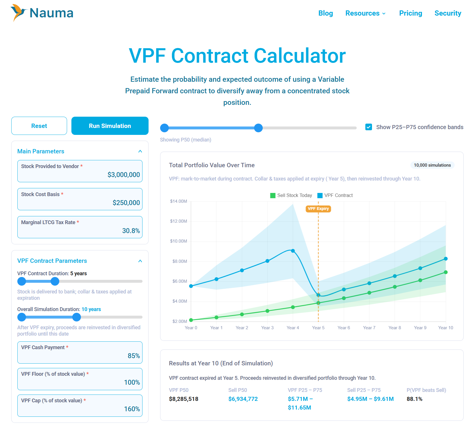
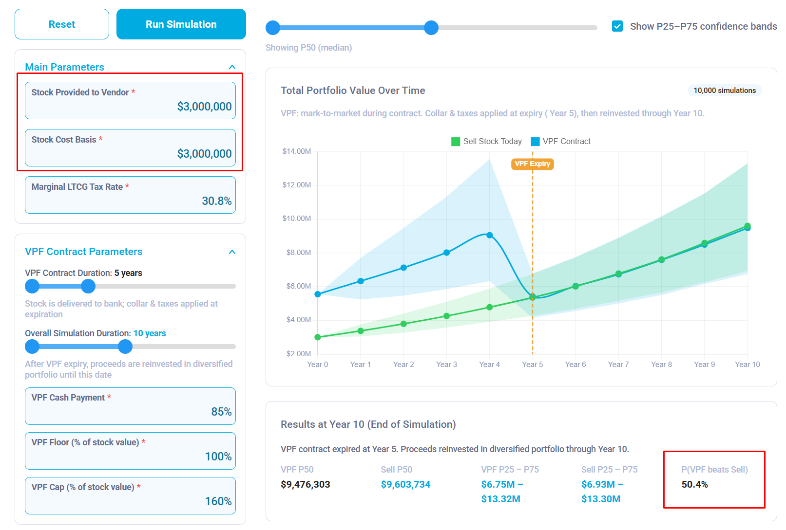
The calculator has three sections for input parameters. Each of them impacts the probability of the investor increasing their overall returns when using VPF contracts:

Main Parameters include the concentrated stock current value, cost basis and marginal LTCG tax rate. These parameters define the benefit of delaying paying capital gains. In the current version of the calculator we assume the current and future LTCG tax rates are the same, but in reality they may differ. Lower future tax rate significantly increases the benefit of VPF.
VPF Contract Parameters: You get them from the bank when you negotiate the terms. You can use SOFR Swap rates as an implied interest rate and then convert that into cash payment for a given VPF contract duration. Floor and Cap are parameters of the Collar.
Market Assumptions: Both concentrated stock and diversified portfolio expected returns & volatility impact the probability of the investor making money when using VPF contracts. The S&P 500 historical data is used for diversified portfolio default values. As I show it below, correlation between concentrated stock and diversified portfolio also affects the results.

The right panel shows a few charts:

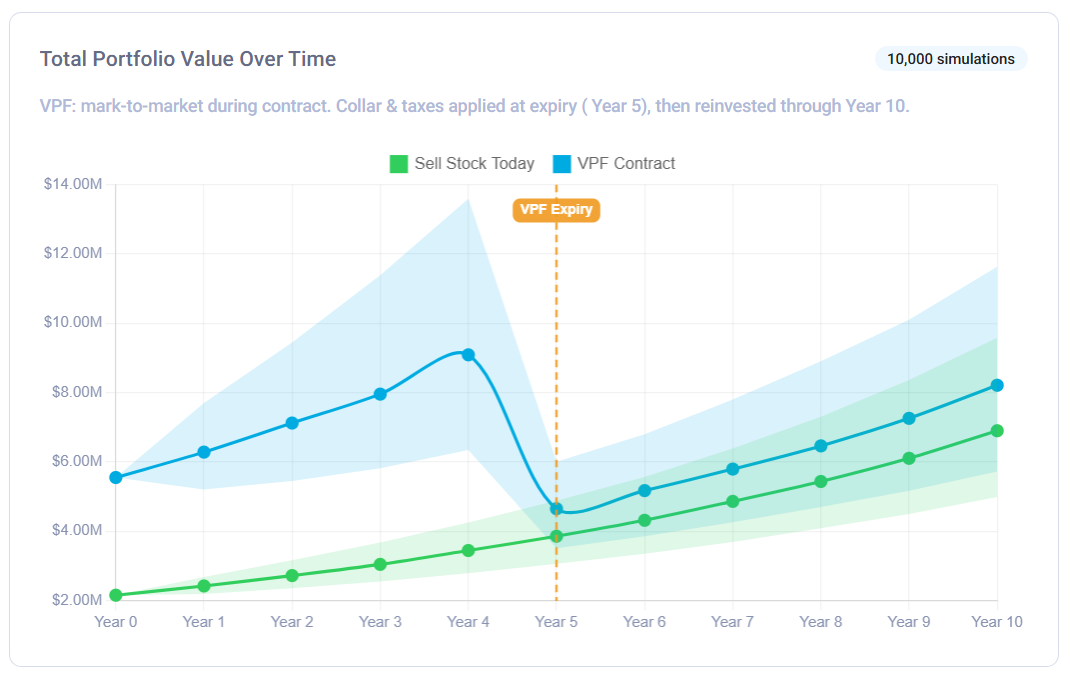
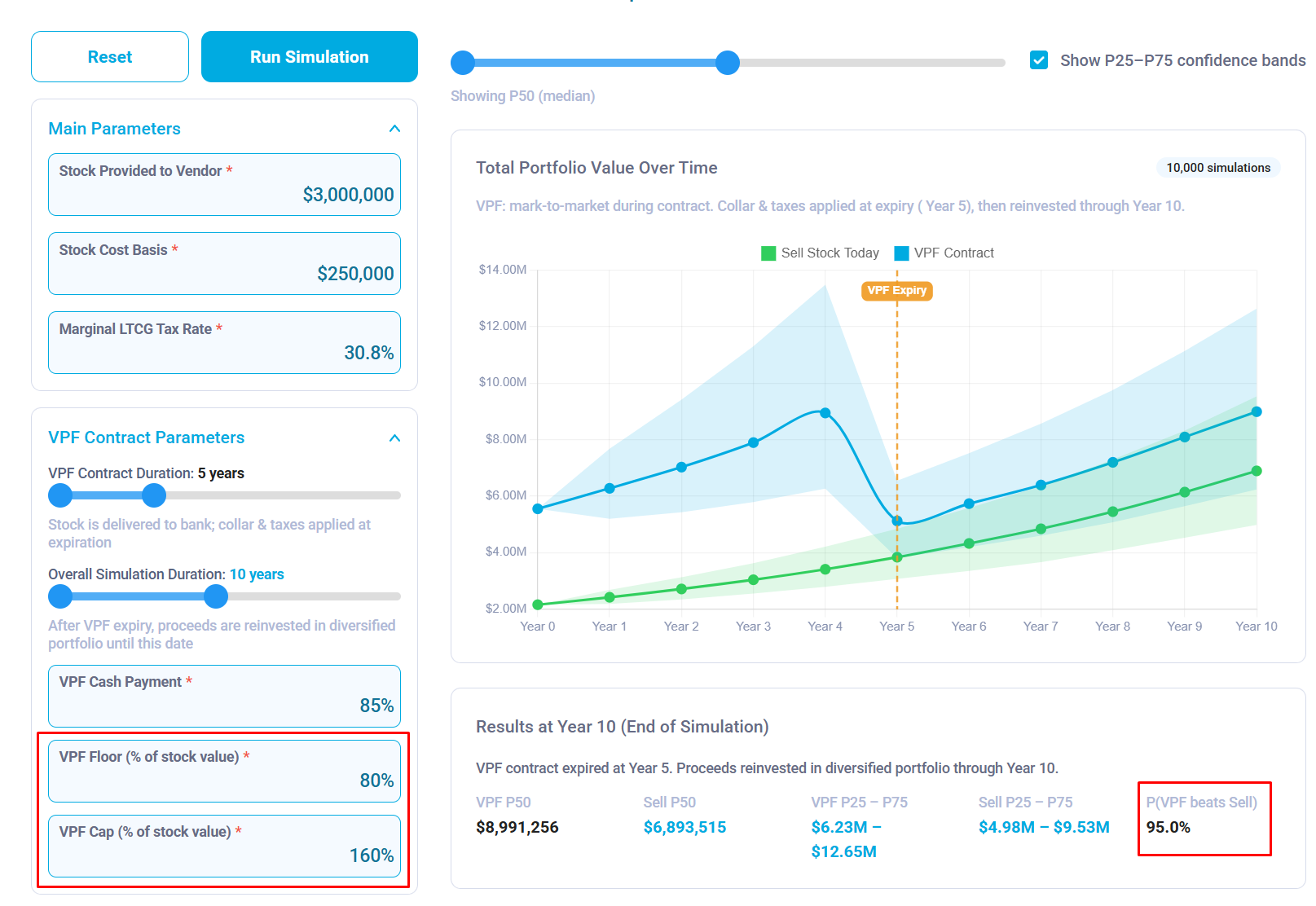
Total Portfolio Value Over Time includes both concentrated stock and diversified portfolio value for VPF contract. Technically, the concentrated stock remains the part of your portfolio until it’s delivered to the bank.
Liquid Portfolio Value Over Time chart excludes the concentrated stock, but you can notice spikes in VPF portfolio value at “VPF Expiry” year. It’s caused by additional concentrated stock profit and taxes.
Liquid Portfolio Annual Return and Liquid Portfolio Annual Volatility: using monte carlo results we calculate average (mean) portfolio return and volatility. Monte Carlo is configured to run 10K simulations.

Annual Volatility Chart demonstrates the spike at “VPF Expiry” year I was discussing above:

The most important value we’ll be looking at when analyzing different VPF parameters is P(VPF beats Sell): probability that the investor makes more money when using a VPF contract. It represents the % of monte carlo runs when the VPF portfolio ended up having more money than a simple sale.

Important insights

Experimenting with model parameters gives us a few important insights which help us understand how VPF contracts work and avoid mistakes when negotiating contract terms with banks:

Concentrated Stock Expected Growth Rate: Using VPF contract makes sense only if the investor believes that the concentrated stock will continue to grow over the next N years. If we set both return and volatility to 0% for concentrated stock, P(VPF beats Sell) = 30.5% for the given set of parameters.

Why: delaying capital gains is beneficial if saved money continues to grow.

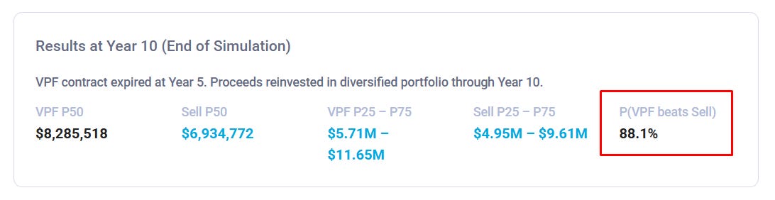
Duration of the VPF contract. Longer VPF contract duration increases the chances of the investor making money.

2 Year contract: P(VPF beats Sell) = 65.5%
4 Year contract: P(VPF beats Sell) = 83.0%
6 Year contract: P(VPF beats Sell) = 92.0%
8 Year contract: P(VPF beats Sell) = 95.7%

Why: Longer durations maximize the benefit of tax deferral. The longer you delay the capital gains tax, the more time your ‘prepaid’ cash has to compound in a diversified portfolio.

Important: VPF Cash Payment will reduce as the duration of VPF contract increases. The real P will probably be lower.

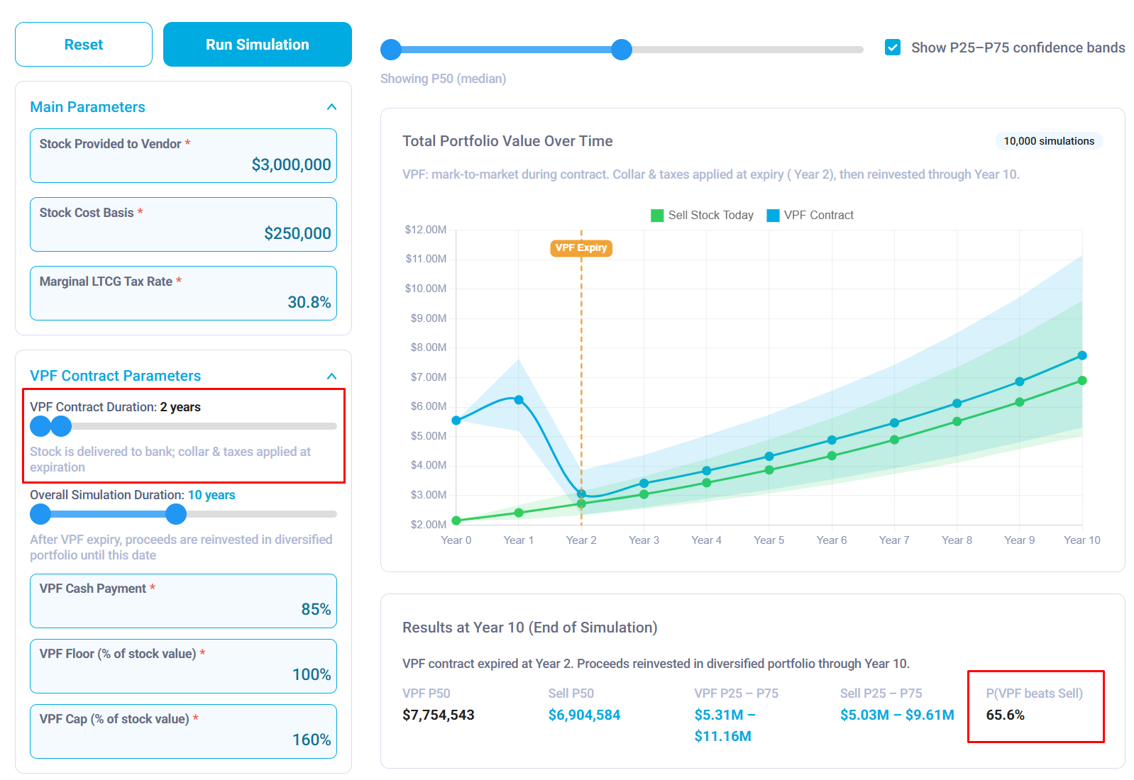
Cost Basis of Concentrated Stock. VPF is more beneficial for concentrated stock with a low cost basis and investors with high marginal LTCG tax brackets. For the default parameters:

$250K Cost Basis: P(VPF beats Sell) = 87.9%
$1M Cost Basis: P(VPF beats Sell) = 80.8%
$2M Cost Basis: P(VPF beats Sell) = 63.1%
$3M Cost Basis: P(VPF beats Sell) = 50.4% (~ coin flip)

Why: the lower cost basis, the higher taxes we pay when we sell the stock.

Floor, Cap and Cash Payment. Lowering the Floor (the strike price of the put protection) appears to increase the probability of success in the model:

100% VPF Floor: P(VPF beats Sell) = 88.3%
80% VPF Floor: P(VPF beats Sell) = 95.0%

In practice, it doesn’t happen. In the real world, the Floor, Cap, and Cash Payment act as three corners of a triangle. If you move one, the others must move to compensate.

The bank’s upfront cash payment is essentially the Present Value (PV) of the Floor.

A 100% Floor means the bank is collateralizing the full current value of the stock, allowing them to give you a higher cash payment (85-90%).
An 80% Floor means you are only collateralizing 80% of the value. In this scenario, the bank will give you significantly less cash upfront (65-70%).

It is very easy for a bank to offer terms that look ‘safer’ on the surface but actually undermine the strategy, making it less likely that the VPF will outperform a simple sale. When evaluating a contract, never look at the Cap or Floor in isolation, always treat the Prepaid Cash Percentage and the Floor as a linked pair.

VPF & Financial Planning

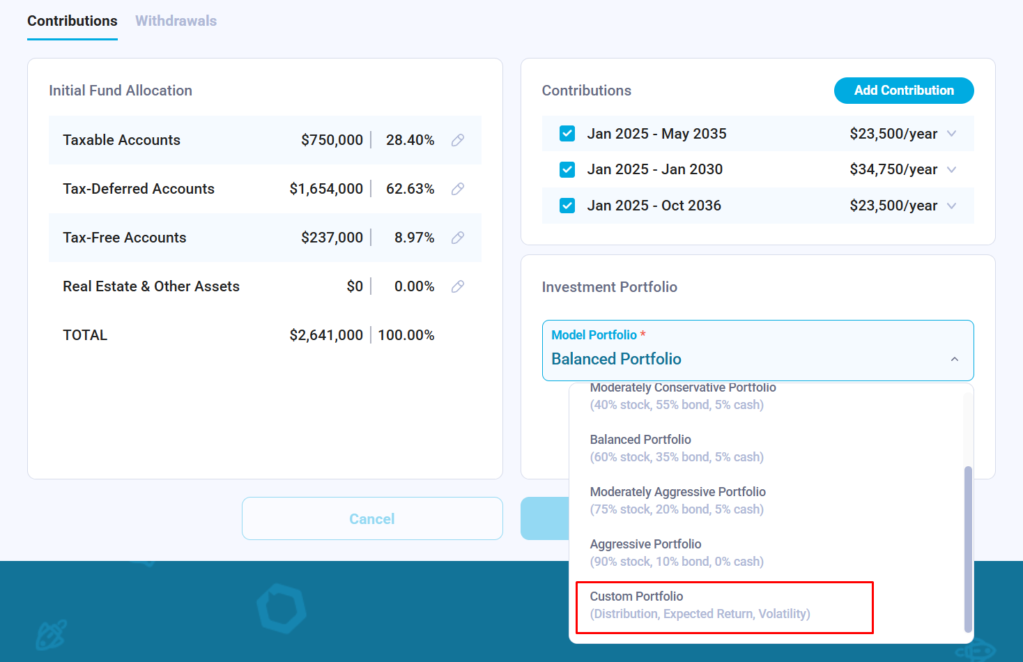
Now when we understand how expected returns and volatility change over time when using VPF contracts, we can start integrating this strategy into our financial plan. I believe that the right approach to integrate complex tax planning strategies in a financial plan is importing calculated expected return and volatility for each year and then testing that portfolio in a Monte Carlo simulation against expected contributions & withdrawals and initial fund allocation.

Conclusion

Navigating the intersection of tax optimization and retirement readiness requires moving beyond the static assumptions of traditional financial modeling. As we have explored, VPF contracts introduce a unique volatility profile, characterized by a period of relative stability in the liquid portfolio followed by a sharp “settlement spike” at expiry.

The Monte Carlo analysis highlights that the effectiveness of a VPF is not a binary “good or bad” decision; it is a highly sensitive calculation that depends on your specific cost basis, the duration of the contract, and the negotiated collar terms.

Ultimately, VPFs are sophisticated tools for deferred tax liability management and leveraged diversification, but they cannot exist in a vacuum. Integrating year-by-year volatility and return expectations into a holistic financial plan is the only way to ensure that while you are optimizing for taxes today, you are also protecting your lifestyle against the sequence of returns risk.

About the Author: Alex Sukhanov, founder of Nauma, a financial planning platform built for people in tech and high-net-worth families. Alex previously worked at Google and started Nauma to help more people in tech make better financial decisions and achieve more in their lives. You can reach out to Alex on linkedin.

Nauma is supported entirely by its users with no commissions and no affiliate incentives. It is designed to give people clarity on taxes, equity compensation and retirement planning.